기계 학습의 기본 개념과 지도·비지도 학습, 모델 평가 과정을 정리합니다.

11장 : 기계 학습

11.1 모델링

개념 : 다양한 변수 간의 수학적 (혹은 확률적) 관계를 표현한 것
예시
- SNS 상에서 사용자수, 사용자당 광고수익 → 차후 몇년 간의 연간 수익
- 요리책에서 먹는 사람의 수, 배고픈 정도 → 재료의 양
- 미국 경기지표, 미국 주식 지표 → 한국 주가 지수

11.2 기계 학습

정의 : 데이터를 통해 모델을 만들고 사용하는 것
예측 모델링, 데이터 마이닝이라고도 불린다.
보통 주어진 데이터로 모델을 구축하고, 새로운 데이터에 만들어진 모델을 적용하면 다음과 같이 다양한 것을 예측해볼수 있다
- 이메일이 스팸 메일인지 아닌지 예측
- 신용카드 사기 예측
- 쇼핑 고객이 클릭할 확률이 높은 광고 예측
- 슈퍼볼에서 우승할 미국 축구팀 예측

<종류>

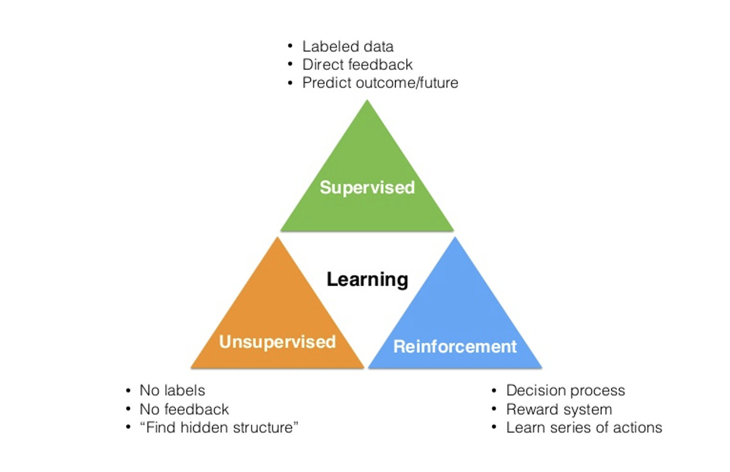
지도 학습 : 학습에 사용될 데이터에 답(종속 변수 값)이 포함되어있는 학습
비지도 학습 : 답(종속 변수값) 이 없는 데이터를 활용해 학습
준지도 학습 : 답(종속 변수값) 이 일부에만 있는 데이터를 활용
온라인 학습 : 새로 들어오는 데이터를 통해 모델을 끊임 없이 조정
강화 학습 : 연속된 예측 뒤 모델이 얼마나 잘 예측 했는지 파악 후 모델을 조정

11.3 Overfitting 과 Underfitting

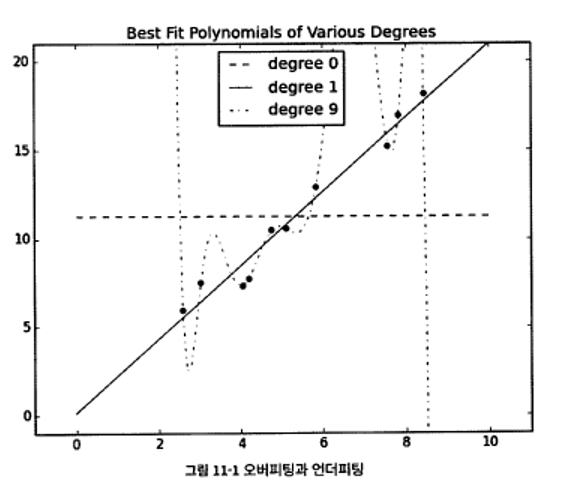
Overfitting (오버피팅)
- 기계 학습의 일반적인 문제점
- 만들어진 데이터모델이 학습데이터에서는 좋지만 새로운 데이터에서는 좋지 않은 경우
- 원인 : 학습 데이터의 잡음이나 불필요한 데이터를 모델에 학습 반영
- 문제점 : 새로운 데이터에 대한 예측의 부적확성
- 예시 : 옆 그림의 9차 함수 (점선)
Underfitting (언더피팅)
- 만들어진 데이터 모델의 성능이 학습 데이터에서도 좋지 않은 경우
- 원인 : 부적합한 모델 선택, 모델을 변경해야 함
- 문제점 : 학습 데이터도 부정확한 예측
- 예시 : 아래 그림의 상수 함수 (가로 점선)

적합 모델을 찾기 위한 실험 설계

적합 모델 찾기 : 학습과 평가 (테스팅) → 학습 데이터와 테스트 데이터의 분할

모델 실험 설계

hold-out 기법

전체 데이터에서 7:3 또는 8:2 등 비율로 훈련 데이터와 테스트 데이터로 나눈다

훈련 데이터(training set)는 모델을 개발하기 위해, 테스트 데이터(test set)는 모델을 평가하기 위해 사용
k-묶음 교차검증

전체 데이터를 k-묶음으로 나눈 후 (k-1)개 묶음

hold-out + validation 기법

검증 데이터 셋을 추가하여, 훈련 데이터에 다시 hold-out 기법을 적용한 방법

검증 데이터셋은 훈련 데이터로 개발된 여러 모델의 성능을 비교하는데 사용되며, 선정된 최선의 모델의 성능은 테스트 데이터셋을 이용하여 평가

hold-out 방식으로 데이터 분할

import random
from typing import TypeVar, List, Tuple

X = TypeVar('X')

def split_data(data: List[X], prob: float) -> Tuple[List[X], List[X]]:
    # 데이터를 섞지 않고 나누는 함수
    idx = int(len(data) * prob)  # 데이터를 나누는 인덱스 계산
    return data[:idx], data[idx:]  # 데이터를 나누어 반환

data = [n for n in range(1000)]  # 0부터 999까지의 숫자로 이루어진 데이터 생성
train, test = split_data(data, 0.75)  # 데이터를 나눔

# 반환된 데이터의 길이가 올바른지 확인
assert len(train) == 750
assert len(test) == 250

# 반환된 데이터가 원본 데이터를 포함하고 있는지 확인
assert sorted(train + test) == data

독립(x), 종속(y) 형태의 데이터 분할

학습 데이터, 평가 데이터에 x와 y가 제대로 쌍을 이뤄서 들어갈수 있도록 한다.

Y = TypeVar('Y')    # 출력 변수를 표현하기 위한 일반적인 타입

def train_test_split(xs: List[X],
                    ys: List[Y],
                    test_pct: float) -> Tuple[List[X], List[X], List[Y], List[Y]]:

    # Generate the indices and split them.
    idxs = [i for i in range(len(xs))]
    train_idxs, test_idxs = split_data(idxs, 1 - test_pct)

    return ([xs[i] for i in train_idxs],  # x_train
            [xs[i] for i in test_idxs],   # x_test
            [ys[i] for i in train_idxs],  # y_train
            [ys[i] for i in test_idxs])   # y_test

xs = [x for x in range(20)]    # xs are 1 ... 1000
ys = [2 * x for x in xs]       # each y_i is twice
x_train, x_test, y_train, y_test = train_test_split(xs, ys, 0.25)

print(xs, ys)
print(x_train, x_test)
print(y_train, y_test)

# 비율이 맞는지 확인
assert len(x_train) == len(y_train) == 750
assert len(x_train) == len(y_test) == 250

# 대응되는 데이터들이 잘 짝지어졌는지 확인
assert all(y == 2 * x for x, y in zip(x_train, y_train))
assert all(y == 2 * x for x, y in zip(x_test, y_test))

# 모델 학습 하고, 성능 평가
model = SomeKindOfModel()
x_train, x_test, y_train, y_test = train_test_split(xs, ys, 0.33)
model.train(x_train, y_train)
performance = model.test(x_test, y_test)

[sklearn.model\_selection.](https://scikit-learn.org/stable/modules/generated/sklearn.model_selection.train_test_split.html)[train\_test\_split](https://scikit-learn.org/stable/modules/generated/sklearn.model_selection.train_test_split.html)[(\*](https://scikit-learn.org/stable/modules/generated/sklearn.model_selection.train_test_split.html)[arrays](https://scikit-learn.org/stable/modules/generated/sklearn.model_selection.train_test_split.html)[, ](https://scikit-learn.org/stable/modules/generated/sklearn.model_selection.train_test_split.html)[test\_size=None](https://scikit-learn.org/stable/modules/generated/sklearn.model_selection.train_test_split.html)[, ](https://scikit-learn.org/stable/modules/generated/sklearn.model_selection.train_test_split.html)[train\_size=None](https://scikit-learn.org/stable/modules/generated/sklearn.model_selection.train_test_split.html)[, ](https://scikit-learn.org/stable/modules/generated/sklearn.model_selection.train_test_split.html)[random\_state=None](https://scikit-learn.org/stable/modules/generated/sklearn.model_selection.train_test_split.html)[, ](https://scikit-learn.org/stable/modules/generated/sklearn.model_selection.train_test_split.html)[shuffle=True](https://scikit-learn.org/stable/modules/generated/sklearn.model_selection.train_test_split.html)[, ](https://scikit-learn.org/stable/modules/generated/sklearn.model_selection.train_test_split.html)[stratify=None](https://scikit-learn.org/stable/modules/generated/sklearn.model_selection.train_test_split.html)[)](https://scikit-learn.org/stable/modules/generated/sklearn.model_selection.train_test_split.html)

Split arrays or matrices into random train and test subsets
Param

test_size, train_size: *float (0.0~1.) or int, default=None*
Returns

splitting*list, length=2 * len(arrays)*

11.4 정확도

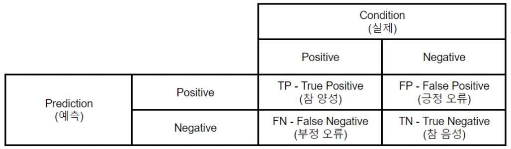
모델의 분류와 정답

True Positive(TP) : 실제 Positive인 정답을 Positive라고 예측 (정답)
False Positive(FP) : 실제 Negative인 정답을 Positive라고 예측 (오답)
False Negative(FN) : 실제 Positive인 정답을 Negative라고 예측 (오답)
True Negative(TN) : 실제 Negative인 정답을 Negative라고 예측 (정답)

정확도 (accuracy)

accuracy = (tp + tn) / (tp + fp + fn + tn)
높게 나와도 의미가 없을 수 있음
정밀도(Precision) : Positive 라고 분류한 것 중에서 실제 Positive 인 것의 비율
재현율(Recall) : 실제 Positive 인 것 중에서 모델이 Positive라고 예측한 것의 비율
특이도(Specificity) : 실제 Negative 중 맞춘 Negative(TN)의 비율
위양성율(FRP : False Positive Rate) : 실제 Negative 중 틀린 Positive(FP)의 비율
위음성율(FNR : False Negative Rate) : 실제 Positive 중 틀린 Negative(FN)의 비율
환자 적용
- 실제 확자를 환자로 판단하는 비율 : Recall, Sensitvity, HitRate
- 실제 환자를 비환자로 판단하는 비율 : FNR
- 비환자(건강한 사람)을 환자로 판단하는 비율 : FPR
- 비환자(건강한 사람)을 비환자로 판단하는 비율 : Specifity
정밀도와 재현율의 트레이드 오프 관계
- 정밀도를 높이려면 가급적 FP가 작아야 한다 → 가급적 negative로 예측해야 함
- 재현율을 높이려면 가급적 FN이 작아야한다 → 가급적 positive로 예측해야 함
조화 평균
- 주어진 수들의 역수와 산술평균의 역수
- 정밀도와 재현율의 조화 평균

[데이터 사이언스] 기계 학습